Evaluating the frequency and common drivers of within-host priority effects during coinfection

Fletcher W Halliday1†, Tuomas Aivelo†, Pablo Beldomenico†, Aaron Blackwell†, Vanessa Ezenwa†, Anna Jolles†, Erin Gorsich†, Claudia Fichtel†, Charlotte Defolie†, Anni M Hämäläinen†, Josue H Rakotoniaina†, Eva Kaesler†, Corey Freeman-Gallant†, Michael Huffman†, Natalie Olifers†, Arnaldo M Júnior†, Elisa P de Araujo†, Rita de Cassia Bianchi†,  Ana PN Gomes†, Paulo HD Cançado†, Matthew E Gompper†, & Paulo S D’Andrea†, Miroslava Soldanova†, Christopher Taylor†, Jason R Rohr

† contributed dataset

1Department of Evolutionary Biology and Environmental Studies, University of Zurich, Zurich, CH

See the poster here.

Download the pdf of this document here.


A current frontier in disease ecology is understanding how interactions among parasite species influence their epidemics. Interactions among parasites can result when prior infection by one parasite alters host susceptibility to a second parasite, generating priority effects among parasite species within host individuals. The increasing number of laboratory studies that aim to measure priority effects highlights growing interest among disease ecologists to understand these processes. Yet, laboratory studies, which are implemented at the scale of host individuals, are poorly suited to understand parasite epidemics, which occur at the scale of host populations, posing a key challenge for disease ecologists. One way to overcome this challenge is to mark and then repeatedly recapture sentinel hosts in the field, then analyze the resulting data using longitudinal regression models (Fenton et al. 2014; Hellard et al. 2015; Halliday et al. 2017, 2018). The purpose of this project was to implement this approach across empirical systems to test two broad questions:

  1. Is disease risk influenced by infection sequence during natural epidemics (i.e., do parasites generally experience/exhibit priority effects)?
  2. To what extent do these within-host priority effects depend on traits of individual parasite species?

To evaluate the role of within-host priority effects during parasite epidemics, we compiled longitudinal datasets of coinfection in host individuals across 13 host and 110 parasite species, including over 25,000 observations of host plants, primates, ungulates, small mammals, birds, and invertebrates. To evaluate the role of within-host priority effects, we performed time-until event analysis, specifically testing whether infection sequence among co-occurring parasites influenced their risk of infection (e.g., Halliday et al. 2017, 2019).  Surprisingly, the sequence of infection predicted fewer than 10% of the more than 1000 pairwise combinations of potentially interacting parasites. This rarity of within-host priority effects may result from a lack of natural variation in infection sequence, indicating that within-host priority effects may be a less common driver of parasite epidemics than previously thought, and highlighting the need for experimental manipulations of parasite infection in the field (e.g., Ezenwa & Jolles 2015; Pedersen & Fenton 2015; Halliday et al. 2017). Showing weak support for ecological theory, parasites with a high degree of niche overlap were slightly more sensitive to priority effects than parasites with a low degree of niche overlap, and this effect was stronger for parasites with narrow niche requirements than with wide niche-requirements. However, in contrast with theory, the frequency of priority effects could not be explained by a parasite’s impact on its host. Together, these results indicate that priority effects may be less commonly detected during natural epidemics than previously expected, and that within-host priority effects among parasites may not necessarily follow the same ecological rules of community assembly as their free-living counterparts.

 The database:

We compiled a database of longitudinal surveys of host individuals (i.e., mark-recapture data), where hosts were unmanipulated (sentinels were ok), and surveyed for infection by multiple parasites. This study focused on interspecific interactions among parasites rather than intraspecific interactions among strains of the same parasite species. The final database includes plants, invertebrate, and vertebrate hosts (Table 1).

Table 1. Contributing authors and associated host datasets
Contributors Host species Host taxon
T. Aivelo Microcebus rufus Primate
P. Beldomenico Hydrochoerus hydrochaeris Rodent
A. Blackwell Homo sapiens Human
V. Ezenwa, A. Jolles, E. Gorsich Syncerus caffer Wild ungulate
AM Hämäläinen, JH Rakotoniaina, E. Kaesler, C. Kraus, P. Kappeler Microcebus murinus Primate
C. Fichtel, C. Defolie Eulemur rufifrons Primate
C. Freeman-Gallant Geothlypis trichas Bird
F. Halliday Festuca arundinacea Plant
M. Huffman Pan troglodytes Primate
N. Olifers, AM Júnior, EP de Araujo , R de Cassia Bianchi,  APN Gomes, PHD Cançado, ME Gompper, & PS D’Andrea Nasua nasua &              Cerdocyon thous Carnivore
M. Soldanova Lymnaea stagnalis Invertebrate
C. Taylor Microtus agrestis Rodent


A standard measurement of within-host priority effects across systems:

To facilitate comparisons across systems, data were analyzed using a common analytical method (described in Halliday et al 2017). Briefly, to detect priority effects, we recorded the sequence of infection by each parasite on each host individual. Time in days since the first survey of each host individual was used as a proxy for exposure to parasite propagules. To model within-host priority effects, we constructed a series of models following Halliday et al (2017). These models explicitly measure priority effects by testing whether the sequence of infection on an individual host influences the rate of infection by each parasite. Each model included one dependent variable pertaining to one parasite species (“the focal parasite”).  To explicitly model priority effects, we used Cox Regression with Firth’s Penalized Likelihood to reduce bias from factors exhibiting (quasi)complete separation (Heinze & Schemper 2002) from the R package, coxphf (Ploner & Heinze 2015), to estimate the probability of a host transitioning from uninfected to infected. Specifically, the dependent variable in each model was time to infection, modeled as the transition rate from uninfected to infected as a function of exposure time. We modeled time to infection resulting from a baseline rate of infection shared by all individuals and modified by the infection status of the host by each other parasite during the previous survey (treated as a time-varying coefficient). Exponentiated coefficients are interpreted as multiplicative changes in infection rate, providing a standardized estimate of priority effects across study systems. Statistically significant (p<0.05) positive and negative coefficients were interpreted as evidence of facilitative and antagonistic priority effects, respectively, whereas non-significant coefficients were interpreted as lacking sufficient evidence of a priority effect occurring.

Our hypotheses:

Hypothesis 1 – Niche overlap. Priority effects are expected to occur more commonly among species with a high degree of niche overlap (Vannette & Fukami 2014). A host comprises the entire niche available to parasites during infection (Kuris et al. 1980; Rynkiewicz et al. 2015), and thus coinfecting parasites often exhibit high niche overlap (Sousa & Zoologist 1992; Graham 2008; Seabloom et al. 2015). The degree of niche overlap among parasites may additionally vary depending on whether parasites share common vectors, employ similar feeding strategies, or share infection sites. We hypothesized that such parasites would therefore more commonly experience priority effects.

Hypothesis 2 – Parasite virulence. Priority effects are expected to occur when early arriving species have a high impact on shared resources with later arriving species (Vannette & Fukami 2014). Parasites require host resources for survival, growth, and reproduction (Lafferty & Kuris 2002). We hypothesized that early-arriving parasites that were more damaging to their hosts would more commonly experience priority effects.

Hypothesis 3 – Host breadth. Priority effects are expected occur when the late arriving species have high requirements for shared resources with early arriving species (Vannette & Fukami 2014). Late arriving species with narrow niche requirements may therefore experience the strongest priority effects. For free-living species, the breadth of niche requirements may manifest as generality in a species’ use of habitat types or tolerance to environmental conditions. For parasites, the breadth of niche requirements may be related to host specificity, defined as the ability to infect multiple unrelated host taxa (Barrett et al. 2009; Park et al. 2018). We hypothesized that late-arriving host specialists would therefore more commonly experience priority effects.

Analytical methods

Data analysis was performed using R version 3.5.2 (R Core Team 2015). To test whether parasites that shared similar traits more commonly experienced priority effects (Hypothesis 1), we used a series of generalized linear mixed models using the lme4 package, version 1.1-20 (Bates et al. 2014), treating the source dataset and host species (Table 1) as random intercepts in each model. The dependent variable in each model was whether or not a pairwise combination of parasites exhibited a priority effect (0,1), and the independent variables where whether or not parasites were the same type (e.g., both macroparasites), shared a common infection site (e.g., both gastrointestinal), or shared the same transmission mode (e.g., both tick-vectored).  Data for every trait was not available for every parasite species (Table S1), so in order to maximize the number of studies contributing to the analysis, each independent variable was therefore tested in a separate analysis. We used inverse-variance weighting based on the number of surveys per host to give more explanatory weight to studies with a greater number of surveys of each host individual. However, because this weighting strongly influenced the results of the analyses, we report results from both weighted and unweighted analyses.

To test whether early-arriving parasites that were more damaging to their hosts would more commonly experience priority effects, we again tested whether or not a pairwise combination of parasites exhibited a priority effect, this time as a function of host virulence. We coded host virulence as 1 if the parasite had few reported adverse effects on the host, 2 if the parasite was known to moderately reduce host fitness, and 3 if the parasite was known to seriously impact host survival (e.g., infections frequently leading to host mortality).

To test whether late-arriving host specialists more commonly experienced priority effects, we used a similar, weighted generalized linear mixed model in lme4, testing whether or not a pairwise combination of parasites exhibited a priority effect as a function of the host specificity of the late-arriving parasite (generalist = known to infect more than one host species; specialist = known to infect only a single host species).

We finally tested whether niche-overlap lead to stronger priority effects among late-arriving host specialists by analyzing the interaction coefficient for each pairwise combination of parasites as a dependent variable.  Because more closely related species tend to exhibit higher niche-overlap, we used the phylogenetic relatedness of parasites as a metric of niche-overlap, and modeled its interaction with host specificity of the late-arriving parasite and their main effects as independent variables in this analysis. Parasites were defined as “closely related” if they shared at least the same order, and “distantly related” if they were from different orders or more distantly related.

Results

Contrary to expectations, we found surprisingly limited evidence of priority effects across our database. Specifically, out of 1128 potential pairwise interactions, we detected only 98 interactions resulting from prior infection (i.e., priority effects). 64 were facilitative (prior infection by one parasite species facilitated subsequent infection by another species), 34 interactions were antagonistic (prior infection by one parasite species inhibited infection by a subsequent species), and the remaining 1030 lacked sufficient evidence to support a priority effect occurring. This surprising result may stem from a lack of variation in infection sequence among study systems. Early infections were often dominated by one or a few parasite species (Fig. 1), potentially resulting from variation in parasite phenology (Halliday et al. 2017) or variation in parasite transmission rates (Clay et al. 2019). Together, these results point to the need for studies that systematically manipulate infection sequence during natural epidemics, potentially through the use of pesticides or anti-parasite treatments of hosts (Pedersen & Fenton 2015).


first_infection_plot_4col
Fig 1. In most study systems, early infections were dominated by one or a few parasites. This lack of variation in infection sequence may explain why fewer priority effects were observed than expected based on laboratory studies. Each point represents a single parasite species, and the y-axis represents the proportion of hosts whose first infection was associated with that parasite. Values on the y-axis sum to >1 due to simultaneous infections.

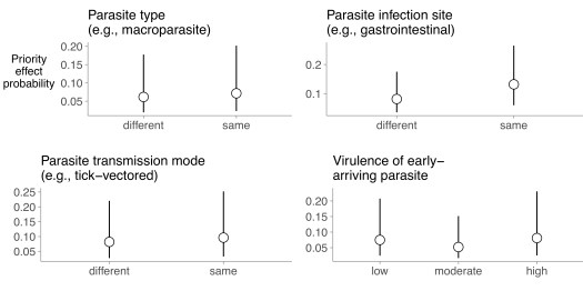
We found weak support for the hypothesis that parasites with high niche overlap would more commonly experience priority effects. Specifically, when weighted by the number of samples per host individual, parasites of the same type (e.g., both macroparasites), parasites that infected the same site (e.g., gastrointestinal parasites), and parasites with the same transmission mode (e.g., both tick vectored), all experienced significantly more priority effects than parasites of different types, different sites, and different transmission modes (p= 0.006, p<0.001, and p = 0.004, respectively; Fig 2). However, these effects were of small magnitude and were not statistically significant when the same analyses were performed with unweighted data (p = 0.98, p = 0.48, p = 0.68, respectively). We found no support for the hypothesis that early-arriving parasites that were more damaging to their hosts would more commonly experience priority effects. Even though the weighted regression indicated that parasite virulence significantly predicted the priority effects (p < 0.001), the direction of this effect was not consistent with our prediction, with moderately virulent parasites exhibiting the lowest rate of priority effects (Fig 2). The effect of host virulence on the probability of observing a priority effect was not significant when the analysis was performed with unweighted data (p = 0.25).


hypothesis_1_3_short
Fig 2. Priority effects were somewhat more commonly observed among parasites of the same type, infection site, or transmission mode (p0.05 when unweighted), lending some support to hypothesis one. In contrast with hypothesis one, priority effects were no more commonly observed when early arriving species had greater or smaller impacts on their hosts, though weighted regression indicates that moderately viulent parasites may exhibit fewer priority effects than low- or highly virulent parasites.

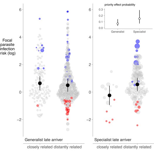
We found strong evidence that later arriving parasites with narrow host breadth (e.g., specialists) more commonly experienced priority effects than parasites with wider host breadth (e.g., generalists; weigthed p < 0.001, unweighted p = 0.007; Fig. 3 – inset). Furthermore, among host specialists, more closely related parasites tended to exhibit more antagonistic interactions (p = 0.003). Together, these results indicate that priority effects among parasites may be less common than expected based on laboratory studies, and that priority effects are rarely consistent with predictions from ecological theory.


plot_with_inset_no_annotation
Fig 3. Priority effects were more commonly observed when late-arriving parasites were host specialists, supporting hypothesis two. Among specialists, more closely related parasites tended to experience more competition. Black circles are model estimated means, error bars are 95% confidence intervals; colored points are estimates from each individual pairwise combination of studies, with size corresponding to the number of samples per host individual. Blue indicates significant facilitation, red indicates significant antagonism, and grey indicates insufficient evidence for significant priority effect. The inset shows the model estimated probability of a priority effect on the y-axis as a function of host specificity.


References

Barrett, L.G., Kniskern, J.M., Bodenhausen, N., Zhang, W. & Bergelson, J. (2009). Continua of specificity and virulence in plant host–pathogen interactions: causes and consequences. New Phytol., 183, 513–529.

Bates, D., Mächler, M., Bolker, B. & Walker, S. (2014). Fitting Linear Mixed-Effects Models using lme4. J. Stat. Softw., 67, 1–48.

Clay, P.A., Cortez, M.H., Duffy, M.A. & Rudolf, V.H.W. (2019). Priority effects within coinfected hosts can drive unexpected population‐scale patterns of parasite prevalence. Oikos, 128, 571–583.

Ezenwa, V. & Jolles, A. (2015). Opposite effects of anthelmintic treatment on microbial infection at individual versus population scales. Science (80-. ).

Fenton, A., Knowles, S.C.L., Petchey, O.L. & Pedersen, A.B. (2014). The reliability of observational approaches for detecting interspecific parasite interactions: comparison with experimental results. Int. J. Parasitol., 44, 437–45.

Graham, A.L. (2008). Ecological rules governing helminth-microparasite coinfection. Proc. Natl. Acad. Sci. U. S. A., 105, 566–70.

Halliday, F.W., Heckman, R.W., Wilfahrt, P.A. & Mitchell, C.E. (2019). Past is prologue: host community assembly and the risk of infectious disease over time. Ecol. Lett., 22, 138–148.

Halliday, F.W., Umbanhowar, J. & Mitchell, C.E. (2017). Interactions among symbionts operate across scales to influence parasite epidemics. Ecol. Lett., 20, 1285–1294.

Halliday, F.W., Umbanhowar, J. & Mitchell, C.E. (2018). A host immune hormone modifies parasite species interactions and epidemics: insights from a field manipulation. Proc. R. Soc. B Biol. Sci., 285, 20182075.

Heinze, G. & Schemper, M. (2002). A solution to the problem of separation in logistic regression. Stat. Med., 21, 2409–2419.

Hellard, E., Fouchet, D., Vavre, F. & Pontier, D. (2015). Parasite-Parasite Interactions in the Wild: How To Detect Them? Trends Parasitol.

Kuris, A.M., Blaustein, A.R. & Alio, J.J. (1980). Hosts as Islands. Am. Nat., 116, 570–586.

Lafferty, K.D. & Kuris, A.M. (2002). Trophic strategies, animal diversity and body size. Tree, 17, 507–513.

Park, A.W., Farrell, M.J., Schmidt, J.P., Huang, S., Dallas, T.A., Pappalardo, P., et al. (2018). Characterizing the phylogenetic specialism-generalism spectrum of mammal parasites. Proc. R. Soc. B Biol. Sci., 285, 20172613.

Pedersen, A.B. & Fenton, A. (2015). The role of antiparasite treatment experiments in assessing the impact of parasites on wildlife. Trends Parasitol., 31, 200–11.

Ploner, M. & Heinze, G. (2015). coxphf: Cox regression with Firth’s penalized likelihood. R Found. Stat. Comput.

R Core Team. (2015). R: a language and environment for statistical computing | GBIF.ORG.

Rynkiewicz, E.C., Pedersen, A.B. & Fenton, A. (2015). An ecosystem approach to understanding and managing within-host parasite community dynamics. Trends Parasitol., 31, 212–221.

Seabloom, E.W., Borer, E.T., Gross, K., Kendig, A.E., Lacroix, C., Mitchell, C.E., et al. (2015). The community ecology of pathogens: Coinfection, coexistence and community composition. Ecol. Lett., 18, 401–415.

Sousa, W.P. & Zoologist, A. (1992). Interspecific Interactions among Larval Trematode Parasites of Freshwater and Marine Snails Interspecific Interactions Among Larval Trematode Parasites of Freshwater and Marine Snails1. Interactions, 32, 583–592.

Vannette, R.L. & Fukami, T. (2014). Historical contingency in species interactions: Towards niche-based predictions. Ecol. Lett., 17, 115–124.

Table S1. Parasites and their associated traits

Parasite Type Virulence Specialist Route Mode Helminth Intracellular
Anaplasma centrale microparasite Low Generalist Complex Tick vectored Not Helminth Intracellular
Ascaris lumbricoides macroparasite Low Specialist Direct Ingestion Helminth Not intracellular
Anaplasma marginale microparasite Medium Generalist Complex Tick vectored Not Helminth Intracellular
Anaplasma phagocytophilum microparasite Medium Generalist Complex Tick vectored Not Helminth Intracellular
Acanthocephala macroparasite Low Complex Ingestion Helminth Not intracellular
Amblyomma cajennense ectoparasite Low Generalist Direct Free-living Not Helminth Not intracellular
Amblyomma ovale ectoparasite Low Generalist Direct Free-living Not Helminth Not intracellular
Amblyomma parvum ectoparasite Low Generalist Direct Free-living Not Helminth Not intracellular
Apicomplexa microparasite Low Complex Not Helminth Intracellular
Ascaridae macroparasite Low Direct Ingestion Helminth Not intracellular
Ascaridida macroparasite Low Direct Ingestion Helminth Not intracellular
Aspidoderidae macroparasite Low Direct Ingestion Helminth Not intracellular
Australapatemon burti macroparasite Medium Generalist Complex Ingestion Helminth Not intracellular
Australapatemon minor macroparasite Medium Generalist Complex Ingestion Helminth Not intracellular
Babesia microparasite Low Generalist Complex Tick vectored Not Helminth Intracellular
Ballantidium microparasite Low Direct Ingestion Not Helminth Not intracellular
Bartonella microparasite Medium Generalist Complex Flea vectored Not Helminth Intracellular
Brucella abortus microparasite Medium Generalist Direct Ingestion Not Helminth Intracellular
Callistoura macroparasite Low Direct Ingestion Helminth Not intracellular
Capillaria macroparasite Low Complex Ingestion Helminth Not intracellular
Cestoda macroparasite Low Complex Ingestion Helminth Not intracellular
Conoidasida microparasite Low Direct Ingestion Not Helminth Intracellular
Colletotrichum cereale microparasite Low Generalist Direct Rain splash Not Helminth Not intracellular
Cooperia macroparasite Low Generalist Direct Ingestion Helminth Not intracellular
Cotylurus cornutus macroparasite Medium Generalist Complex Ingestion Helminth Not intracellular
Cowpox virus microparasite Medium Generalist Direct Direct contact Not Helminth Intracellular
Dicrocoeliidae macroparasite Low Generalist Complex Ingestion Helminth Not intracellular
Diphyllobothriidae macroparasite Low Complex Ingestion Helminth Not intracellular
Diplostomum pseudospathaceum macroparasite Low Generalist Complex Ingestion Helminth Not intracellular
Dipylidiidae macroparasite Low Complex Ingestion Helminth Not intracellular
Ehrlichia ruminantium microparasite Medium Generalist Complex Tick vectored Not Helminth Intracellular
Anaplasma microparasite Low Specialist Complex Tick vectored Not Helminth Intracellular
Echinocleus hydrochaeri macroparasite Low Specialist Complex Ingestion Helminth Not intracellular
Echinoparyphium aconiatum macroparasite Medium Generalist Complex Ingestion Helminth Not intracellular
Echinoparyphium recurvatum macroparasite Medium Generalist Complex Ingestion Helminth Not intracellular
Echinostoma revolutum macroparasite Medium Generalist Complex Ingestion Helminth Not intracellular
Eimeria boliviensis microparasite Medium Specialist Direct Ingestion Not Helminth Intracellular
Eimeria hydrochaeri microparasite Medium Specialist Direct Ingestion Not Helminth Intracellular
Eimeria microparasite Medium Specialist Direct Ingestion Not Helminth Intracellular
Entamoeba microparasite Medium Direct Ingestion Not Helminth Not intracellular
Fasciolidae macroparasite Low Generalist Complex Ingestion Helminth Not intracellular
Siphonaptera ectoparasite Low Generalist Direct Free-living Not Helminth Not intracellular
Giardia lamblia microparasite Medium Generalist Direct Ingestion Not Helminth Not intracellular
Haemonchus macroparasite Medium Direct Ingestion Helminth Not intracellular
Ancylostomatidae macroparasite Low Specialist Direct Free-living Helminth Not intracellular
Hymenolepis macroparasite Low Generalist Complex Ingestion Helminth Not intracellular
Hypoderaeum conoideum macroparasite Low Generalist Complex Ingestion Helminth Not intracellular
Laelapidae ectoparasite Low Direct Free-living Not Helminth Not intracellular
Lemuricola macroparasite Low Specialist Direct Ingestion Helminth Not intracellular
Lemurostrongylus macroparasite Low Specialist Direct Ingestion Helminth Not intracellular
Leucocytozoon microparasite Low Generalist Complex Blackfly vectored Not Helminth Intracellular
Listrophorus ectoparasite Low Generalist Direct Free-living Not Helminth Not intracellular
Phthiraptera ectoparasite Low Generalist Direct Free-living Not Helminth Not intracellular
Metagonymus macroparasite Low Generalist Complex Ingestion Helminth Not intracellular
Hystrichopsyllidae ectoparasite Low Generalist Direct Free-living Not Helminth Not intracellular
Moliniella anceps macroparasite Low Generalist Complex Ingestion Helminth Not intracellular
Myobiidae ectoparasite Low Generalist Direct Free-living Not Helminth Not intracellular
Neotrichodectes pallidus ectoparasite Low Specialist Direct Free-living Not Helminth Not intracellular
Notocotylus attenuatus macroparasite Low Generalist Complex Ingestion Helminth Not intracellular
Oesophagostomum macroparasite Medium Generalist Direct Ingestion Helminth Not intracellular
Opisthioglyphe ranae macroparasite Low Generalist Complex Ingestion Helminth Not intracellular
Opisthorchis macroparasite Low Generalist Complex Ingestion Helminth Not intracellular
Oesophagostomum stephanostomum macroparasite Medium Generalist Direct Ingestion Helminth Not intracellular
Oxyuridae macroparasite Low Direct Ingestion Helminth Not intracellular
Pararhabdonema macroparasite Low Generalist Direct Ingestion Helminth Not intracellular
Paryphostomum radiatum macroparasite Low Generalist Complex Ingestion Helminth Not intracellular
Physalopteridae macroparasite Low Complex Ingestion Helminth Not intracellular
Plagiorchis elegans macroparasite Low Specialist Complex Ingestion Helminth Not intracellular
Plasmodium microparasite Medium Specialist Complex Mosquito vectored Not Helminth Intracellular
Protozoophaga obesa macroparasite Low Specialist Direct Ingestion Helminth Not intracellular
Strongyloides macroparasite Low Generalist Direct Free-living Helminth Not intracellular
Caenorhabditis macroparasite Low Direct Ingestion Helminth Not intracellular
Strongyloidae macroparasite Low Generalist Direct Ingestion Helminth Not intracellular
Chromadorea macroparasite Low Helminth Not intracellular
Enterobius macroparasite Low Direct Ingestion Helminth Not intracellular
Panagrellus macroparasite Low Direct Ingestion Helminth Not intracellular
Puccinia coronata microparasite Low Specialist Complex Airborne Not Helminth Not intracellular
Rhizoctonia solani macroparasite Medium Generalist Direct Rain splash Not Helminth Not intracellular
Schistosoma macroparasite Medium Generalist Complex Free-living Helminth Not intracellular
Schistosomatidae macroparasite Medium Generalist Complex Free-living Helminth Not intracellular
Strongyloides fuelleborni macroparasite Low Generalist Direct Ingestion Helminth Not intracellular
Strongiloides macroparasite Low Generalist Complex Free-living Helminth Not intracellular
Strongyloidae macroparasite Low Generalist Complex Free-living Helminth Not intracellular
Strongiloides chapini macroparasite Low Generalist Complex Free-living Helminth Not intracellular
Subulura macroparasite Low Complex Ingestion Helminth Not intracellular
Theileria mutans microparasite Low Generalist Complex Tick vectored Not Helminth Intracellular
Theileria parva microparasite High Generalist Complex Tick vectored Not Helminth Intracellular
Theileria sable microparasite Low Generalist Complex Tick vectored Not Helminth Intracellular
Theileria sp (buffalo) microparasite Medium Generalist Complex Tick vectored Not Helminth Intracellular
Trichuris trichiura macroparasite Low Specialist Direct Ingestion Helminth Not intracellular
Theileria velifera microparasite Low Generalist Complex Tick vectored Not Helminth Intracellular
Mycobacterium tuberculosis microparasite Medium Specialist Direct Airborne Not Helminth Intracellular
Thysanotaenia macroparasite Low Specialist Complex Ingestion Helminth Not intracellular
Ixodida ectoparasite Low Generalist Direct Free-living Not Helminth Not intracellular
Trematoda macroparasite Low Complex Helminth Not intracellular
Trichinellidae macroparasite Low Complex Ingestion Helminth Not intracellular
Trichobilharzia szidati macroparasite Low Generalist Complex Free-living Helminth Not intracellular
Trichodectes canis ectoparasite Low Generalist Direct Free-living Not Helminth Not intracellular
Trichostrongyloidea macroparasite Low Direct Ingestion Helminth Not intracellular
Trichuris macroparasite Low Specialist Direct Ingestion Helminth Not intracellular
Trichuris cutillasae macroparasite Low Specialist Direct Ingestion Helminth Not intracellular
Trichuris macroparasite Low Specialist Direct Ingestion Helminth Not intracellular
Trypanosoma microparasite Medium Generalist Complex Tsetse fly vectored Not Helminth Intracellular
Trichuris trichiura macroparasite Low Specialist Direct Ingestion Helminth Not intracellular


Even deleting the chestnut blight won’t necessarily bring the chestnut tree back*

This post was originally published on BioDiverse Perspectives – a research blog aimed at fostering communication about biodiversity.

100 years ago, the Eastern United States was a lot different than it is today.  Yeah, there was less urban development, and there were fewer paved roads, dams, and railroads, but by far the biggest difference (at least to an ecologist) was the makeup of the forests.  100 years ago, there stood a huge and dominant tree that is now a mere shrub.  Prior to 1904, the mighty chestnut was one of the most dominant trees in the entire northeast, comprising as much as 40% of the canopy.  Chestnuts grew up to five feet in diameter, and up to 100 feet tall, provided some of the best lumber, and produced some of the most valuable nuts to people and wildlife. But in 1904 in New York City, some chestnuts began to die.  The blight, caused by the introduced fungus, Cryphonectria parasitica, quickly invaded North American forests as it encountered American trees with little natural resistance, girdling and eventually killing them.  By the 1920’s, Cryphonectria had spread to the Appalachian forests and was quickly heading south, and by the 1930’s, the blight had entirely removed chestnuts from the southern Appalachian forests (McCormick and Platt 1980).

Twenty years after the demise of of the chestnut, researchers saw no evidence that it could ever recover, and until now they have been right. But what if the chestnut got a second chance?  What if suddenly and unexpectedly, Cryphonectria disappeared in the temperate deciduous forests of North America?  Because Cryphonectria appears to have been the only initial factor limiting the growth and abundance of chestnut, it is reasonable to believe that if it were to disappear, chestnut populations could recover back to their pre-blight status. And had humans contributed little else to change the forests since the early 20th century, disappearance of Cryphonectria could have as great an effect on Eastern US forests it had twenty years after its arrival to North America.   However, due to current and past land-use, chestnut interacts with a different suite of co-occurring species and must contend with a shifting climate. Therefore, while deleting Cryphonectria may change deciduous forests, it would do little to restore the chestnut as a dominant species.

To illustrate my point, lets delve a little more into the biology of the pathogen and the host.

What is Cryphonectria?

Crhyphonectria, a member of the phylum Ascomycota, grows on the shoots of Castanea.  The mycelium produces a canker inside the bark of the tree, and once the canker has encircled the entire stem, it girdles and kills it.  This leads to the death of the majority of the tree. But Cryphonectria never enters the roots, leaving them intact to produce shoots known as stump-sprouts.  As a result, chestnut is reduced to an understory shrub rather than being completely eked out.

What does this mean for the chestnut?  It means that with the disappearance of Cryphonectria, Chestnuts would not have to rely solely on seed dispersal to begin returning back into the forests.

A Closer Look at the Chestnut Tree, Castanea

The chestnut is a highly efficient seed disperser. And this may be one of the primary factors that contributed to the past dominance of the Chestnut tree in North American forests.  Chestnut seeds are nuts, which are protected by a thick husk that allows the seeds to survive past their most vulnerable stage to one that is more conducive to dispersal.  Chestnuts also produce massive quantities of seeds, and they produce them mid-summer, which protects the nuts from the potential impacts of frost.  The nuts are also highly palatable and rapidly harvested by animals, which aids in dispersal. This means that if chestnuts could grow large enough to produce seeds and become abundant enough to overcome seed predation, they could potentially proliferate quickly towards forest dominance. And because Castanea can produce shoots from already existing (and rather abundant) root stock, they should be able to produce seeds quickly, relative to reestablishing from seed.

What happened to North American deciduous forests after the Chestnuts died?

We don’t know a lot about chestnut ecology before the blight, but thanks to one plot of land on Beanfield Mountain, we know something about how forests responded to the chestnut’s demise. Prior to the blight, Castanea was a co-dominant species in all the sloped forests of Beanfield Mountain.  In 1939, about twenty years after introduction of Chestnut Blight to the mountain, the only perceptible difference in composition was the absence of chestnut. After about 50 years, openings in the forest canopy were eventually filled by hickory, as Eastern US forests shifted from chestnut/oak to oak-hickory dominated. Then, largely due to fire-exclusion during the early 20th century, populations of red maple invaded forests, and now red maple is one of the most abundant trees in eastern forests (Lord 2004).

How did chestnuts get to North America last time?

Long before they were deciduous, North America was home to boreal forests.  Then, around 16,000 years ago in the south, and 10,000 years ago further to the north, deciduous forest began to take over the landscape. But Castanea was the slowest species of tree to establish, expanding at roughly 100 meters per year, and reaching sites near Connecticut only as recently as 2,000 years ago, even though it was present near Memphis 13,000 years prior.  Margaret Davis (1983) suggested that that despite high seed production and dispersal, the fact that Castanea is self-sterile could be a leading factor for such a slow rate of establishment, and still account for the huge proliferation once established.

What does this mean for the chestnut tree?

What does this tell us about reestablishment of chestnut following the disappearance of Chryphonectria?  First, though chestnuts are not currently producing seed, they do so rapidly, yet they distribute very slowly as a species.  Second, despite their slow dispersal, they still exist in many areas as small shrubs awaiting an opportunity to grow.  And third red maple is their primary competitor in a world without chestnut blight.

 Factors Limiting Reestablishment of Castanea

Ok, you’re saying, the chestnut’s chances don’t sound so dire. They are already in forests, and they produce massive quantities of seed when mature. What’s the deal?

Plant competition for light is asymmetrical.  With a large enough canopy, trees can effectively block sunlight from reaching the branches of lower plants, slowing growth and seed production.  The chestnut has been reduced to an understory shrub. And although plants can survive for decades in the shade, and despite being widely considered one of the fastest growing canopy trees in the Appalachian forest when under direct sunlight, the chestnut’s growth is heavily stunted by shade (Bass 2002).  As a result, despite release from Chryphonectria, it would take chestnuts decades to grow large enough to produce seed and widely disperse throughout the forests.

Red maple, a current forest dominant, is one of the most sensitive forest trees to burning, and periodic fires resulting from Native American activities, lightning strikes and European settling practices were likely key factors in suppressing red maple populations in the past.  Perhaps with the re-introduction of fire into Eastern US Forests, canopy openings could allow new chestnut stump-shoots to grow and become dominant.  Sadly, current fire practices would need to change on a scale beyond any we’ve seen before, and so it appears that despite an absence of Cryphonectria as a shoot limiting factor, the red maple will still limit chestnut growth in its absence.

And human fire practices are not the only factors keeping chestnut trees in check.  As a result of the excessive killing of Wolves in the past, deer populations have increased. And because deer tend to choose other shoots over red maple (Abrams 1998), there could be a problem of excessive deer browsing of chestnut shoots were they able to grow to substantial size and health.  This could further deter them from recolonizing the forests and give the red maple another advantage.

Last, tree reestablishment would have to contend with shifting climate regimes.  Suppose chestnut trees were able to overcome the shading from red maple and preferential selection by browsers. They might be able at maximum growth, to reach half the height of the canopy in twenty years, and reach the full height in 80 (Bass 2002).  But in 80 years will current North American forests still be the ideal location for Chestnut trees?  It was once predicted that range extensions due to climate would require a dispersal rate over 200km per century, that’s over 2km per year (Davis, 1989).  With a dispersal rate of 100m per year, it seems unlikely that Castanea could keep up with increasing temperatures.

It’s sad to think that our introduction of Cryphonectria over 100 years ago, failed to serve as an effective warning, and that through historical resource use, we managed to prevent the forests from being successfully reinhabited by a once dominant and majestic tree.


Want more information about Chestnut blight and the chestnut tree? Check out these resources:

Bass Q. 2002. Talking Trees: The Appalachian Forest Ecoysystem and the American Chestnut. The Journal of The American Chestnut Foundation 16:42-55.

Davis M. B. 1983. Quaternary History of Deciduous Forests of Eastern North America and Europe. Annals of the Missouri Botanical Garden 70:550-563.

Delcourt H. R. 1979. Late Quaternary Vegetation History of the Eastern Highland Rim and Adjacent Cumberland Plateau of Tennessee. Ecological Monographs 49:255-280.

Keever C. 1953. Present Composition of Some Stands of the Former Oak-Chestnut Forest in the Southern Blue Ridge Mountains. Ecology 34:44-54.

Lord B. 2004. The Red Maple, An Important Rival of the Chestnut. The Journal of The American Chestnut Foundation 18:42-47.

McCormick J. F., R. B. Platt. 1980. Recovery of an Appalachian Forest Following the Chestnut Blight or Catherine Keever-You Were Right! American Midland Naturalist 104:264-273.

Paillet F. L. 2002. Chestnut: history and ecology of a transformed species. Journal of Biogeography 29:1517-1530.

Steele, M.A., McCarthy, B.C. & C. H. Keiffer. 2005. Seed Dispersal, Seed Predation, and the American Chestnut. The Journal of The American Chestnut Foundation 19:47-55.

VANDER WALL S. B. 2001. The Botanical Review; The Evolutionary Ecology of Nut Dispersal. 67:74.

Woods F. W., R. E. Shanks. 1959. Natural Replacement of Chestnut by Other Species in the Great Smoky Mountains National Park. Ecology 40:349-361.


*Disclaimer: This post is largely plagiarized from a paper that I wrote as an undergraduate, which is one reason why it’s so long, and also may explain why the citations are so old.

Advice to prospective graduate students

This post was originally published on BioDiverse Perspectives – a research blog aimed at fostering communication about biodiversity.

Getting into grad school is a lot of work. By now, most North American PhD programs in ecology are in the “recruitment phase”. Students have already taken their GRE entrance exams, contacted professors, obtained letters of recommendation, written applications, and waited. Soon they will be visiting prospective universities for the dreaded interview weekend. Below is a list of things (originally published in 2014) that we wish we’d known going into grad-school recruitment. Got others? Share them in the comments section below.

I’ll be the first to admit that I didn’t know much going into graduate school interviews. What I did know was that a commitment to grad school is more than a commitment to a program. I knew that I’d be committing to a relationship with people – especially my potential advisor and lab mates – and that I’d be committing to a relationship with a geographical location – between high school and grad school, I’d never lived in one place for longer than 3 years (thanks in part to an extended stay in junior college), so this was a big deal for me. My eventual recruitment trips reflected this. I asked a lot of questions about grad student – advisor relationships, and I asked a lot of questions about the places I was visiting. Here are some things I didn’t really think about, though:

  1. Try to get to know your potential advisor. A bad relationship with your advisor can poison your grad school experience. And although asking fellow grad students about their relationships can be useful, your relationship with your new advisor is going to be a reflection of your two personalities. No two relationships are the same, so use this opportunity to get to know your potential advisor as best you can.
  2. The same thing goes for getting know a place. One of the things I truly regret not taking advantage of while I was interviewing was the opportunity to travel. If you have time, stay a couple extra days and check out your potential future home.
  3. Take control of your spare time. Recruitment weekends can be really hectic, especially if you end up with a day of back-to-back-to-back interviews. If you need a break, do it. For me, this meant reminding myself that it was okay to stop and use the bathroom between meetings, even if said bathroom breaks weren’t scheduled. I guess an alternative could be to invest in a stadium pal.
  4. Finally ask your hosts about the questions they wish they had asked. In addition to providing some good advice, this can also be a nice window into the hopes and regrets of grad students who have made the exact decision that you’re contemplating. A group of fantastic grad students in the biology department at UNC put together this handy list of things to talk to your potential advisor about before you accept a position in their lab. Who knows, maybe your host has put something like this together, too. -Fletcher Halliday

When I made the decision to start a PhD program, I had the advantage of having already obtained a masters’ degree and taking time off (2.5 years) from grad school. From this perspective I knew something that I think most, particularly young fresh-from-undergrad applicants, don’t take seriously enough when making a final decision on what program to attend. That is, the whole ‘life’ picture – strike a balance between a program and a place that will allow you to achieve balance (when you have time!). Grad school is super intense and stressful. If you end up at an awesome school that is in an awful and unfriendly town your work could ultimately suffer because of it (and vice versa!). While at recruitment take the time to scope out life outside the walls of the university. Definitely ask current students how they feel about the area and what they do for fun. I really feel many don’t think through how their personal-side of life will look during grad school. Don’t assume you can compromise personal happiness, particularly in a program that may last 4-8 years! -Kylla Benes

When you’re visiting a lab, take some time to meet the other grad students.  Whether you become best friends or not, if you join their lab you’ll be spending plenty of time with these people.  Also, these are people who have gone through the same process you are, and have been accepted to a lab and (hopefully) feel happy there.  If you’re visiting for more than a day, go out for dinner and beers with them, and ask them every single question you can think of.  What’s it really like working in their lab?  Is the professor nice or is he or she a jerk?  Do they micromanage or do they expect their students to be independent?  How long do most graduate students take to graduate?  What sorts of jobs do they get afterwards?  How much do grad students make, and how does that compare to the city’s cost of living?  What sorts of things do students do for fun outside of school?  Is there a good social scene (how far away are the bars) or is it a pretty quiet city? Kylla mentioned this already, but I wanted to emphasize how important this question is. You may be surprised with the answers they give, but you’ll definitely be glad you asked. -Nate Johnson

Like Nate, I also encourage you to seek out grad students, ideally as far from campus as possible (I know our institute arranges lunches and/or dinners that are students-only). I’ve found that graduate students are nothing if not candid, especially when it comes time to bitch about their job/lack of pay. So take everything that is said with a grain of salt and ask them straight up “You’ve mentioned a lot of negative things, why are you here?” Also know that their opinion is not the only one: I’ve seen labs where some people absolutely despise their advisor (and labmates), and others in the very same lab get along famously (both with advisors and each other). So don’t get stuck talking to the one disgruntled student, or if you do, know that they are probably using you as an outlet to vent every negative thing they hate about their life.

I also think its important to point out that interviews run both ways: yes, you should be on your best behavior, but so should they. So while it seems like most of the pressure is on you, you hold more of the cards: if they’ve invited you up for the weekend and offered to pay your way, they want you. You have passed muster: your grades are good, your statements were compelling, you demonstrate potential to succeed, and most notably, some faculty has stood up and said “Yes, I will shepherd* them through 3-7 years of intellectual exploration!” (*fund) So relax, take a breath, and enjoy yourself. If you’re more comfortable, you’re also likely to come across better. And don’t be afraid to admit that this advisor/lab/school isn’t for you. I had an interview where I knew pretty much right off the bat that it wasn’t a good fit, on any level. We parted amicably (I hope!) but I wrote the person immediately afterwards and said thank you, I appreciated you taking the time to show me around, but personally I didn’t feel it was a good fit.

Good luck! -Jon Lefcheck

On these trips it’s easy to focus on the faculty and to some extent the grad students in the lab and program. That’s all very valuable, but it’s also a good idea to interact with the other prospectives as well. I definitely DON’T mean being competitive with them, because if you choose to enter that program, some subset of that group will be your cohort, which can be your most valuable asset in getting through grad school. Your peers will help you normalize manuscript rejections, listen to you vent about research frustrations and qualifying exam anxieties. Of course, you don’t know who will and won’t join the program in your interview group, but it’s worthwhile to consider whether they are a group of people you could see yourself spending time with socially (though it’s not necessary) or who you would want to have access to when you need emergency field assistance on the tide flats at 3 am.

And to reiterate what was said above, remember that current grads and faculty can also get burned out by these events. I agree with Jon that everyone should be on their best behavior! But, if they do seem tired or cynical, maybe just remember that it can be an occupational hazard from time to time.

Also, never get intimidated by the process (easier said than done). It’s all about fit, and the timing. These interviews certainly feel like a performance, but you need to be a certain amount of relaxed to be able to take in all the information about the program and people that will help you make a decision about what’s good for you. – Emily Grason


An homage to the writing style of Dr. Peter Adler -Or- How to write good science well.

This post was originally published on BioDiverse Perspectives – a research blog aimed at fostering communication about biodiversity.

Although I’ve been a graduate student for more than four years, I’ve been a peer-reviewed author for just a few short months. My brief time as a researcher, writer, and published scientist in no way makes me an expert when it comes to developing a successful career in academia. However, during my time in grad school, I have become aware of three critical rules for achieving success in my field.

Rule 1. Do good science. This is a no-brainer, really. If you want to be recognized for your contributions to the scientific world, start with good science.
Rule 2. Be an advocate for your science. This is less obvious, but equally important. One of the most critical ways for your good science to be recognized is for you to advocate for it. This means give talks whenever you can, reach out to broad audiences, and most importantly, publish your research.
Rule 3. Communicate your science well. This is the least obvious of these three rules. However, if people can’t understand your good science, it’s unlikely to be recognized for its contribution to the field.

Graduate school puts a huge emphasis on Rule 1 – and for good reason. Grad school is first and foremost a place for young researchers to learn how to do good science, and without good science Rules Two and Three are irrelevant. In my program, Rule 2 is covered pretty well, too. Students get to practice giving talks and presenting posters during departmental brown-bags and an annual research symposium. My lab also encourages me to attend large and small conferences to share my research, and grad students from my department have been encouraged to start and contribute to a number of research blogs.

But Rule 3. That’s a tough one. I mean, how many research faculty were actually trained in science communication? And can they really be expected to teach that skill to graduate students? So to tackle Rule 3, graduate students are pointed to reference books and resources on the Internet. And the Internet is replete with advice on how to write well. For example, see Brian McGill’s 2012 tome on writing clearly  – a follow up to Jeremy Fox’s question who writes the most stylish scientific papers? – And read Brian’s subsequent post on writing journal articles like a fiction author.

While it is tempting to just have someone do your writing for you. That won't get you very far in academia.
While it is tempting to just have someone do your writing for you. That won’t get you very far in academia.


For a recent assignment in a scientific writing seminar, I was encouraged to take a different approach to tackle Rule 3. Find a researcher whose writing you like or admire. Read a few of their scientific papers and identify some characteristics of their writing style and organization (not scientific content) that makes it successful.

For the assignment, I decided to choose an author whose papers I enjoy reading, and who exemplifies the three rules of academic success. And it didn’t take me long to land on Peter Adler. Dr. Adler is widely regarded for his ability to synthesize complex theory with empirical data – He does good science. He gave what I regard as the best talk at ESA 2014, not only because his research findings were interesting and important, but because I left the talk feeling smarter than when it began. – He advocates for his science. Last, Adler’s papers are frequently cited and he is regarded as a clear communicator – He communicates his science well.

And so I set out on a journey to try to figure out how Peter Adler communicates his research. In particular, I wanted to see if I could identify two themes in his papers.

  1. Adler is well regarded for his ability to clearly explain and synthesize complicated theory and modeling approaches with empirical data. Are there any stylistic themes that he uses to accomplish this?
  2. Adler publishes prolifically. Is there any indication for a roadmap that he might use for writing?

To do that, I focused on four papers:

Here I should note that all of these papers have co-authors and it’s a disservice to those coauthors to assume that Adler is the sole contributor to the writing style and ultimate success of the article.

  1. Can I identify stylistic themes that Adler uses to clearly explain and synthesize complex theory / modeling approaches with empirical data.

Adler uses conversational sentence construction with relatively short words. Occasionally rephrases a concept for clarity.

“Stabilizing processes are defined as any mechanism that causes species to limit themselves more than they limit others. Another way of saying this is that niches cause intraspecific effects to be more negative than interspecific effects. As a result, when any one species increases in abundance, its per capita growth rate slows relative to other species, helping to limit competitive exclusion.” (Niche for Neutrality)

Why I think it works: In a perfect world, writing would be maximally concise and clear. However, in the real world, brevity can often come at a cost to clarity. Adler is willing to sacrifice some space for clarity in an instance when it is particularly important that the reader understand a concept. 

He asks questions and then provides an answer

“What precisely are the fitness differences among species that are important from a coexistence perspective? The specific traits depend on the model used to describe coexistence.” (Niche for Neutrality)

“How can functional traits directly affecting only a limited set of physiological processes and demographic rates explain variation in overall life history? One possible explanation is that the affected processes…” (Forecasting plant community impacts) 

Why I think it works: The idea of raising questions and then immediately answering them isn’t new. The literary device even has a name: Hypophora. Why do writers use it? It can help maintain interest and curiosity in a reader, highlight important questions, and guide the reader towards an important area of interest. Why does it work for Adler? Reading Adler’s well-placed questions helps me follow the logic of his argument. He’s both telling me what to ask and the answer to my question.

In a non-research paper, Adler ends each section with a small “take home message”

“Placing the neutral model within classic coexistence theory emphasizes two important lessons…”(Niche for Neutrality)

It then goes on to summarize the two important lessons: (1) that niche and neutral processes combine to generate coexistence, and (2) that relationships between per capita growth rates and relative abundance can allow researchers to test their relative contributions.

Why it works: Non-research papers aren’t required to follow the IMRAD structure that most research papers follow. This can be confusing if early sections of a paper don’t clearly link together until later on. Briefly summarizing each section provides the reader with a reminder of the greater context of each section.

He uses simple language in the introduction and more complex jargon in the methods section.

Intro of Coexsitence of perennial plants, describes stabilizing niche differences as mechanisms that

“cause species to limit themselves more than they limit others, so each species grows faster when it is rare than when it is common.”

In the methods, they are described as,

“all processes that cause species to limit conspecific more than heterospecific individuals, creating an advantage when rare.”

Why it works: This approach allows the reader to understand the concepts early on, but the technical details when they are necessary. In other words, Adler gives the reader just enough information so that they can understand the basic concept in the introduction, but then introduces the technical details of that concept in the methods section, where they are necessary to critically evaluate the research.

Adler makes frequent use of numbered lists to organize ideas.

“Our results provide three important clues to guide future research on specific mechanisms.” (Coexistence of perennial plants)

Why it works: (1) Improves clarity by focusing the reader on key concepts. (2) Increases brevity by eliminating unnecessary transition statements. (3) Provides a framework for following paragraphs

(2) Do Adler’s papers follow a consistent general outline?

The introduction of each paper begins with a broad overview of the theory, the historical approach, the problem, and a new solution.

Why I think it works: The introductory paragraph provides a broad historical context for the rest of the paper. This is essentially an exaggerated version of “The Funnel Introduction technique”.

Each intro ends with a paragraph that outlines the rest of the paper. This paragraph often lists objectives of the paper and summarizes how those objectives were met.

“We begin by fitting… We then perturb the observed climate variables…Next, we estimate the degree of niche differentiation…Finally, we show that this empirical test supports…” (Forecasting plant community impacts)

Why it works: Adler’s research is complicated. At the end of the introduction, he provides the reader with a roadmap. Get lost during the paper? Refer back to the roadmap to find your way.

Each component of the methods section is told as a story:

Why it works: The narrative approach helps the reader understand how each step in data collection and analysis leads to the final result.

The discussion section always begins by restating the objectives.

“Our analysis of the empirical, multispecies population model supported our hypothesis: Species with dynamics strongly stabilized by niche differences experienced the weakest indirect effects of climate, while the species most weakly stabilized by niche differences was most sensitive to indirect effects.” (Forecasting plant community impacts)

Why it works: Like before, restating ideas comes at a cost to brevity. In this case, restating and summarizing the objectives and results increases clarity by highlighting the concepts that the discussion will cover.

Ok, so what’s the take-home message here? It’s not that Peter Adler is the best writer on earth and we should all emulate everything he does. Rather, I think there are two really important messages from this exercise. First, good writing is effortful writing. If your goal is clarity, it is important to think critically about sentence and paragraph construction, not just the logical flow of arguments. I would imagine that it also requires a level of cognitive empathy – or the ability to understand what confuses a reader and make that clear. For example Adler rephrases a difficult concept in Niche for Neutrality to help the reader follow along with the flow of ideas. Second, being a good writer means thinking analytically about writing. What do I mean by that? Grad school trains us to think critically about constructing scientific experiments, statistical tests, logical arguments. Yet thinking critically about constructing sentences and paragraphs is rarely emphasized. Perhaps the trick to accomplishing Rule 3 is to approach it like Rule 1.

Updates from the field: The most abundant species that we know nothing about.

This post was originally published on BioDiverse Perspectives – a research blog aimed at fostering communication about biodiversity.

I’m going to start this post by issuing a challenge: Look at the picture above and identify the most abundant organism. Go ahead, I’ll give you a second. Here’s a bigger version of the picture if that one is too small.

Got it?

“Ok,” you’re saying, “either that was too easy or you’re tricking me.”

Here’s what I see when I look at that picture. I see grassland that’s pretty much dominated by a single grassland species. Since I took the picture, I know that the grassland is in California at the Pepperwood Preserve in Santa Rosa. The grassland species is an exotic grass known as Harding grass (Phalaris aquatica). It is thought to be native to Northern Africa and the Middle East, to have been introduced to California a long time ago, and to have been spread throughout Northern California by the Soil Conservation Corps to prevent erosion. Some might call it an invasive species. So is that it? Is Harding grass the most abundant species in the picture?

Maybe. But what if we enhance the picture?

enhance1


Enhance

IMG_5323


Enhance

HAR02 (1)

There’s a fungus growing on the leaves of Harding grass in Santa Rosa. On each leaf are hundreds (thousands?) of individuals of the rust fungus, Puccinia coronata – each one producing a little pustule. And there can be so many of them during some parts of the year that it’s impossible to walk through the grasslands without your clothes getting covered in spores.

Preserve ecologist, Michelle Halbur, has to worry about becoming a disease vector during grassland monitoring season.

And what’s even more interesting about this fungus is that even though it may be the most abundant organism in this grassland, it’s never been documented here. In fact, according to the USDA, Puccinia coronata has never been documented infecting Harding grass outside of its native range.

And it’s not like researchers don’t know anything about Puccinia coronata or Phalarais aquatica. So how come, despite the availability of research preserves with missions to “steward life and landscapes” and “advance science-based conservation of ecosystems,” have we as researchers failed so completely at describing what may be the most abundant species present? Some might argue that ecologists have a history of under-appreciating the importance and abundance of parasites in the natural world. Others might suggest that Harding grass’s native pathogens are only now starting to catch up after its initial introduction into California. One thing is certain – if we want to understand the ecology of the Pepperwood Preserve, we better start getting to know the ecology of this disease.

***************************************************

It was my first field season of graduate school. I was completely overwhelmed and unsure what I wanted to study, when I came face-to-face with the most abundant species at the Pepperwood Preserve. Great! I’ll describe the pathogen and do some experiments. I’ve found a dissertation! Then I got back from the field. A month passed. I found another dissertation topic. The month turned into a semester – three new dissertation topics. The semester turned into a year, and at five or six dissertation topics post-Puccinia, I started to worry that Pepperwood Preserve’s most abundant species* would never be described.

Unsure how to proceed, but certain that we needed to make progress understanding this pathogen, I reached out to some instructors at Santa Rosa Junior College. They put me in touch with some students, and together, we cobbled together “Puccinia coronata Field Crew 1”. In addition to working towards describing the pathogen, PcFC-1 started to notice some patterns of disease across the landscape. They identified a hypothesis, collected data, analyzed it, and reported results. This year, PcFC-2 has not only kept the project going, but is collecting even more data and testing new hypotheses. And PcFC-2 has gone one step further by submitting an abstract to the Ecological Society of America, where they will present their results in the Friday poster session.

So far, here’s what we know about the most abundant species at Pepperwood Preserve: We know what it is  – Puccinia coronata. We know that infection severity is heterogeneous across space and time. We know that in 2013, there was no effect of host density on infection severity. Through careful observations and collaborations between knowledgeable landowners, professional ecologists, college faculty, and students, Pepperwood has empowered us to make progress towards addressing some of the problems that plague our field. In doing so, we’re joining the next generation of natural historians in revealing the novel ecological systems that have gone undetected right under our noses.

Puccinia coronata Field Crew 1 - led by student Prahlada Papper (front) and faculty member Tony Graziani (back, left) tested the hypothesis that plants that stand taller than the surrounding vegetation are more exposed to pathogens than their shorter relatives.
Puccinia coronata Field Crew 1 – led by student Prahlada Papper (front) and faculty member Tony Graziani (back, left) – tested the hypothesis that plants that stand taller than the surrounding vegetation are more exposed to pathogens than their shorter relatives.


*ok, so the most abundant question was a trick question. And if we’re going to start getting nitpicky about organisms living on organisms, who is to say that there aren’t microbes invisible to the naked eye that are even more abundant than P. coronata? To that, I say – Yes! I totally agree!